Predicting Bank Customer Churn with Machine Learning in R
Introduction

Customer churn, a phenomenon where customers discontinue their business relationship with a company, is a critical challenge faced by organizations across various industries. In the context of the banking sector, where customer relationships are the backbone of sustainable growth, understanding and mitigating customer churn has taken center stage. The financial services landscape is highly competitive, and retaining customers is paramount for a bank's success.
In this era of data-driven decision-making, the ability to identify early signs of customer churn and take proactive measures can make all the difference. Customer acquisition costs can be significantly higher than retaining existing customers, underscoring the need to focus on customer retention strategies. For banks, customer churn can lead to decreased revenues, loss of market share, and a tarnished reputation. The complexity of modern banking, with its myriad of products and services, makes it imperative to delve deep into customer behavior patterns, preferences, and factors influencing churn.
This is where exploratory data analysis (EDA) comes into play. EDA, an essential phase of the data analysis process, involves visually exploring and summarizing data to extract valuable insights. By harnessing the power of EDA, banks can uncover hidden trends, relationships, and anomalies within their customer data that might be contributing to churn. This article delves into the world of bank customer churn and the pivotal role of exploratory data analysis in addressing this challenge. Through a step-by-step approach, we will explore various visualizations and analytical techniques to gain a comprehensive understanding of customer churn and its underlying dynamics. By the end of this article, you will be equipped with insights to help banks make informed decisions that mitigate churn and foster customer loyalty.
Understanding the Problem
In the competitive landscape of the banking industry, customer churn has emerged as a critical concern that directly impacts a bank's profitability and growth trajectory. Customer churn, also known as customer attrition, refers to the phenomenon where customers end their relationship with a company or service provider. For banks, losing customers can translate into reduced revenue, eroded market share, and increased acquisition costs for replacing lost customers. Understanding the drivers and dynamics behind customer churn is crucial for devising effective retention strategies. By identifying the factors that contribute to churn, banks can proactively intervene to retain valuable customers and enhance overall customer satisfaction.
Dataset Overview: In this article, we will leverage a dataset obtained from Kaggle, a renowned platform for data science enthusiasts and practitioners. The dataset contains valuable information about bank customers and various attributes that may influence their decision to churn. The dataset includes details such as customer ID, credit score, country, gender, age, tenure, account balance, number of products, credit card ownership, active membership status, estimated salary, and churn status (whether the customer churned or not).
Data Preparation and Exploration
Before we delve into unraveling the complexities of customer churn through Exploratory Data Analysis (EDA), it's crucial to equip ourselves with the right tools and lay the groundwork. In the code snippet provided, we set the stage for our analysis by loading essential libraries and preparing the dataset.
The journey begins with the inclusion of essential R packages that will empower us throughout the analysis.
PRO TIP: Why pacman?
The utilization of the pacman package in our code snippet brings an additional layer of elegance and clarity to our analysis. While the primary goal of loading libraries is to access their functionalities, the way we manage libraries can significantly impact the readability and maintainability of our code.
Traditional methods of loading libraries involve a series of library() calls, where each library needs to be installed separately if not already present. This can clutter the code. Enter the pacman package, a versatile tool that streamlines the process of library management.
By employing the p_load() function from the pacman package, we condense multiple library() calls into a single line of code. This not only makes our code more concise but also simplifies the management of dependencies. The specified libraries, in our case tidyverse, caTools, caret, pROC, tidyr, reshape2, gridExtra, and randomForest, are not only loaded but are also installed automatically if they are not already installed.
        # Our code without using pacman

        # Install packages
        install.packages("tidyverse")
        install.packages("caTools")
        install.packages("caret")
        install.packages("pROC")
        install.packages("tidyr")
        install.packages("reshape2")
        install.packages("gridExtra")
        install.packages("randomForest")

        # Load libraries
        library(tidyverse)
        library(caTools)
        library(caret)
        library(pROC)
        library(tidyr)
        library(reshape2)
        library(gridExtra)
        library(randomForest)


        # Option B
        # Install required packages
        install.packages(c("tidyverse", "caTools", "caret",
            "pROC", "tidyr", "reshape2", "gridExtra", "randomForest"))

        # This?
        library(c("tidyverse", "caTools", "caret", "pROC", "tidyr",
            "reshape2", "gridExtra", "randomForest"))

        # Unfortunately, library() function does not accept vector inputs

        # Custom function to load packages and install if necessary
        load_and_install_pkgs <- function(pkgs) {
            for (pkg in pkgs) {
                if (!requireNamespace(pkg, quietly = T)) {
                install.packages(pkg, dependencies = T)
                }
                library(pkg, character.only = T)
            }
        }

        # List of packages you want to load
        pkg_to_load <- c("tidyverse", "caTools", "caret", "pROC",
            "tidyr", "reshape2", "gridExtra", "randomForest")

        # Load and install packages
        load_and_install_pkgs(pkg_to_load)
The provided code illustrates various methods for managing R packages. The first approach involves installing and loading packages individually, which can be cumbersome and repetitive. The second approach attempts to install and load multiple packages using vectors, but the `library()` function doesn't accept vector inputs. The third method employs a custom function to iteratively install and load packages, offering some streamlining. However, the most advantageous approach is to use the `pacman` package, which simplifies the process by enabling one-line installation and loading of multiple packages with automatic installation and loading functionalities. This approach offers conciseness, ease of use, and flexibility when managing packages in R.
We utilize the pacman package to ensure that the required libraries (tidyverse, caTools, caret, pROC, tidyr, reshape2, gridExtra, randomForest) are installed and loaded into the environment.
        # Load libraries
        library(pacman)
        p_load(tidyverse, caTools, caret, pROC,
            tidyr, reshape2, gridExtra, randomForest
        )

        # Options
        options(scipen = 999)

        # Load data
        df <- read_csv('Bank Customer Churn Prediction.csv')


        # Data Preprocessing
        str(df)
        summary(df)

        # Display basic information about the dataset
        str(dataset)
        summary(dataset)
Data Preprocessing
        # Data Preprocessing
        str(df)
        summary(df)

        # Checking for NA values
        any_na <- any(is.na(df))

        # Correct data conversion
        df$country <- factor(df$country)
        df$gender <- factor(df$gender)
        df$tenure <- factor(df$tenure)
        df$products_number <- factor(df$products_number)
        df$credit_card <- factor(df$credit_card)
        df$active_member <- factor(df$active_member)
        df$churn <- factor(df$churn)

        summary(df)
Data preprocessing is a critical step to ensure that the data is in the right format and free from errors that could affect the analysis. In this section, we first examine the structure and summary statistics of the dataset using the `str()` and `summary()` functions. We then check for any missing values (NA values) in the dataset.
After identifying the data types and potential missing values, we proceed with data conversion. Categorical variables like 'country,' 'gender,' 'tenure,' 'products_number,' 'credit_card,' 'active_member,' and 'churn' are converted into factors to facilitate analysis and modeling.
Exploratory Data Analysis: Visualizing Customer Churn
In the realm of data analysis, visualizations play a pivotal role in uncovering insights and patterns within a dataset. In this section, we'll delve into the Exploratory Data Analysis (EDA) process, where we'll leverage various types of plots to gain a deeper understanding of customer churn.
Histograms: Exploring Numerical Variables
Histograms are excellent tools to visualize the distribution of numerical variables within a dataset. Let's start by examining key attributes such as age, credit score, account balance, and estimated salary.
            # Age
            ggplot(df,
                aes(
                    x = age
                )
            ) +
            geom_histogram(fill = 'darkgreen', color= 'white')+
            labs(title = "Distribution of Age",
                x = "Age",
                y = "Frequency"
            ) +
            theme_bw() +
            theme(plot.title = element_text(hjust = 0.5))


            # Credit Score
            ggplot(df,
                aes(
                    x = credit_score
                )
            ) +
            geom_histogram(fill = 'darkgreen', color= 'white')+
            labs(title = "Distribution of Credit Score",
                x = "Credit Score",
                y = "Frequency"
            ) +
            theme_bw() +
            theme(plot.title = element_text(hjust = 0.5))

            # Balance
            ggplot(df,
                aes(
                    x = balance
                )
            ) +
            geom_histogram(fill = 'darkgreen', color= 'white')+
            labs(title = "Distribution of Account Balance",
                x = "Account Balance",
                y = "Frequency"
            ) +
            theme_bw() +
            theme(plot.title = element_text(hjust = 0.5))

            # Visualize accounts with balance greater than zero
            df |>
            filter(balance > 0) |>
            ggplot(
                aes(
                x = balance
                )
            ) +
            geom_histogram(fill = 'darkgreen', color= 'white')+
            labs(title = "Distribution of Account Balance",
                x = "Account Balance",
                y = "Frequency"
            ) +
            theme_bw() +
            theme(plot.title = element_text(hjust = 0.5))

            # Estimated Salary
            ggplot(df,
                aes(
                    x = estimated_salary
                )
            ) +
            geom_histogram(bins = 20, fill = 'darkgreen', color= 'white')+
            labs(title = "Distribution of Salary Estimates",
                x = "Estimated Salary",
                y = "Frequency"
            ) +
            theme_bw() +
            theme(plot.title = element_text(hjust = 0.5))
Let us talk about all the plots the code above produced.
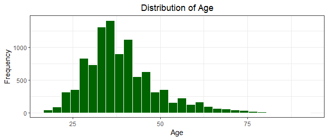
We notice here the bulk of the bank customers are below the age of 45 years, with very few of the customers over 50 years, indicating a youthful customer base.
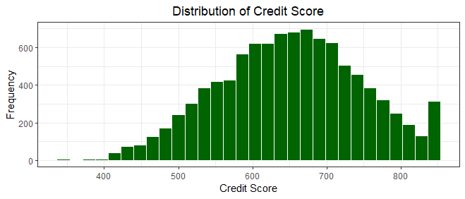
Our histogram showcases a bell-shaped curve, suggesting a relatively symmetrical distribution of credit scores. The majority of customers have credit scores clustered around the center of the range, around 600 - 700, with the highest peak around the median score of 650.
The distribution tails off gradually towards both ends, indicating that very low and very high credit scores are less common. The spread of credit scores from 350 to 850 demonstrates the entire spectrum of creditworthiness, with the mean score of approximately 650.5 indicating a central tendency. However, the presence of some outliers towards the higher end suggests that a small fraction of customers possess exceptionally high credit scores.
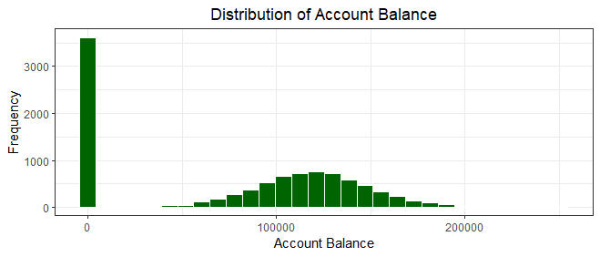
We notice here an unusual number of accounts with a balance of zero and for the purpose of our plot, we used tidyverse's dplyr to filter out all accounts with a balance of zero out to produce a clearer plot as shown below.

After filtering out zero balances, the distribution of account balances in the dataset exhibits a different pattern. The histogram now portrays a somewhat right-skewed distribution, though not as pronounced as before. The majority of customers maintain positive account balances, with a notable peak around the median balance of 119840.
The range of balances spans from 3769 to 250898, reflecting the diversity in customers' financial positions. While the distribution still displays a tendency towards lower balances, the shift away from the zero balance instances has led to a more evenly distributed histogram.
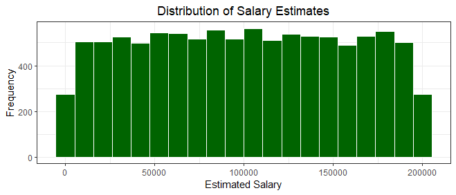
The histogram above showcases a relatively symmetric distribution, resembling a bell-shaped curve. Most customers' estimated salaries are centered around the median value of 101139.30. The range of estimated salaries spans from around 11 to around 190,000, encompassing a diverse range of income levels.
While the majority of customers fall within the middle range of salaries, the distribution gradually tails off towards the higher and lower ends. The relatively symmetrical nature of the histogram suggests that the dataset captures a balanced representation of estimated salaries, with no significant skewness evident.
Barplots: Categorical Variables Overview
Barplots are adept at portraying the distribution of categorical variables. Here, we'll explore the distribution across different countries, credit card ownership, gender, and account status.
            # Country
            ggplot(df,
                aes(
                    x = country
                )) +
            geom_bar(fill='salmon',color= 'black') +
            labs(title = "Distribution of Customers by Country",
                x = "Country",
                y = "Frequency") +
            theme_bw() +
            theme(plot.title = element_text(hjust = 0.5))

            # Number of Bank Products
            ggplot(df,
                aes(
                    x = products_number
                )) +
            geom_bar(fill = 'darkgreen', color= 'white')+
            labs(title = "Distribution of Products",
                x = "Number of Products",
                y = "Frequency") +
            theme_bw() +
            theme(plot.title = element_text(hjust = 0.5))

            # Credit Card
            df$credit_card <- factor(df$credit_card)

            ggplot(df,
                aes(
                    x = credit_card
                    )) +
            geom_bar(fill = 'salmon', color = 'black')+
            labs(
                title = "Distribution of Customers by Credit Card Ownership",
                x = "Credit Card",
                y = "Frequency") +
            theme_bw() +
            theme(plot.title = element_text(hjust = 0.5))


            # Active Member

            ggplot(df,
                aes(
                    x = active_member
                )) +
            geom_bar(fill = 'salmon', color = 'black')+
            labs(
                title = "Distribution of Customers by Account Status",
                x = "Status",
                y = "Frequency") +
            theme_bw() +
            theme(plot.title = element_text(hjust = 0.5))

            # Churn
            # Churn by Country
            ggplot(df, aes(x = country, fill = factor(churn))) +
            geom_bar(position = position_dodge(), color='black') +
            labs(title = "Churn Distribution by Country",
                x = "Country",
                y = "Count") +
            scale_fill_manual(values = c("0" = 'darkgreen', '1' = 'salmon'),
                                name = "Churn",
                                labels = c("Did Not Churn", "Churned")) +
            theme_bw() +
            theme(plot.title = element_text(hjust = 0.5))

            # By Gender
            ggplot(df, aes(x = gender, fill = factor(churn))) +
            geom_bar(position = position_dodge(), color='black') +
            labs(title = 'Churn Distribution by Gender',
                x = 'Gender',
                y = 'Count') +
            scale_fill_manual(values = c("0" = 'darkgreen', "1" = 'salmon'),
                                name = "Churn",
                                labels = c("Did Not Churn", "Churned")) +
            theme_bw() +
            theme(plot.title = element_text(hjust = 0.5))
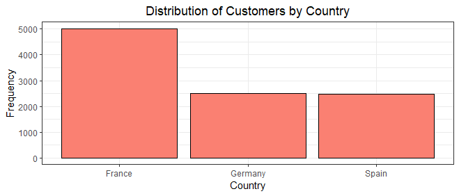
The bar chart above provides a visual representation of how customers are distributed across different countries, shedding light on the frequency of each country's occurrence within the dataset.
Notably, France emerges as the dominant country with the most customers, exhibiting the highest count(5,014) of customers, closely pursued by Germany(2,509) and Spain(2,477).
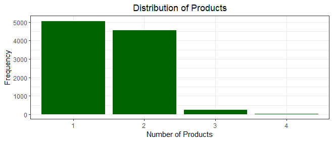
The bar chart depicting the distribution of the number of bank products per customer offers an illuminating view of customer engagement with the bank's offerings. The majority of customers exhibit ownership of either one(5,084 customers) or two(4,590 customers) bank products, with a smaller segment having three(266 customers) or four(60 customers) products.
This visualization offers a snapshot of customers' preferences and needs when it comes to utilizing the bank's array of products. This emphasizes the widespread adoption of a limited number of products among the customer base, indicating a predominant inclination towards a more streamlined banking experience.
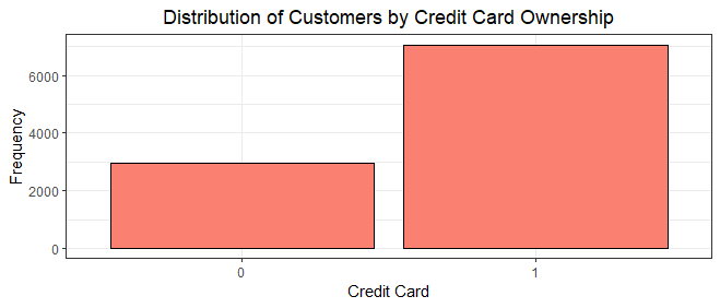
The bar chart illustrating credit card ownership among customers provides a comprehensive glimpse into their financial behaviors. It's evident that a significant portion of customers(7,055 customers) possess credit cards, while a smaller fraction(2,945 customers) does not, underscoring the importance of credit cards as a common and integral aspect of the banking relationships maintained by the customers.
From a churn perspective, the prevalence of credit card ownership could indicate a higher likelihood of retention among customers who actively use the bank's products. Conversely, the absence of credit card ownership might signal a segment with less attachment, potentially warranting closer attention to understand their reasons and mitigate churn risks. This visualization provides an avenue for deeper churn analysis by linking credit card ownership to customer engagement and retention potential.
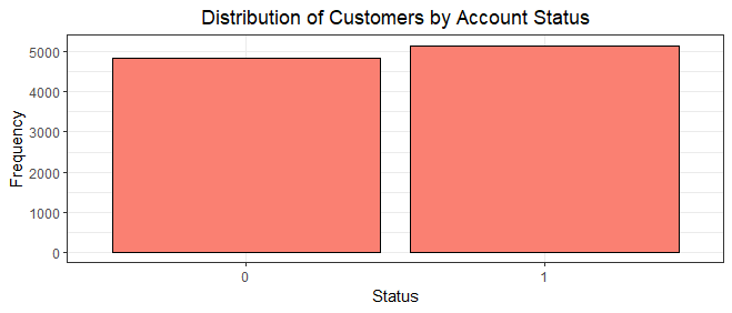
With 5151 active members and 4849 inactive members, the bar chart portrays a more balanced engagement pattern within the customer base. While a majority is still engaged, the gap between active and inactive members is not as pronounced.
This underscores the need for a nuanced approach in understanding customer engagement dynamics. It prompts a closer examination of the factors driving both active and inactive statuses, potentially revealing opportunities to re-engage inactive members and further strengthen relationships with the active ones.
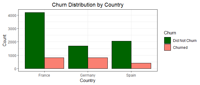
From our plot above, we can see Germany, the country with the least customers, recorded the highest churn volume out of the other two countries, and even more than France, a country with almost double Germany's customer base.
This is unusual and might prompt the bank to investigate furtheras to the driving factors behind the underperformance in Germany. Spain recorded the lowest churn rate, with less than 25% of its customer base churning.
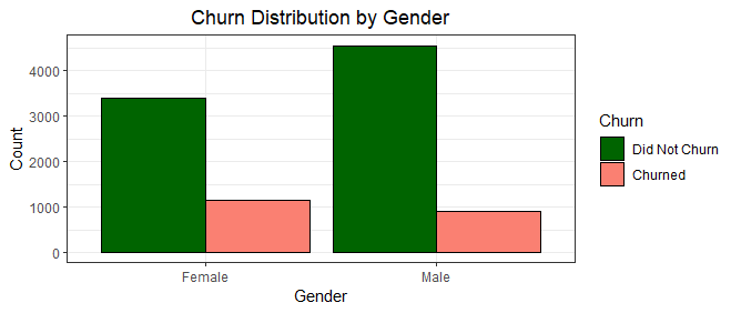
When it comes to churn rate by gender, females recorded a higher churn rate than males, despite it being the lesser gender composition of the bank's customer base.
Boxplots: Understanding Churn Patterns
Boxplots are powerful tools to comprehend the distribution and variability of data, especially in relation to categorical variables. In this section, we focus on understanding churn patterns based on country, gender, age, credit score, account balance, and estimated salary.
            # Dashboard
            # Churn by Age
            p1 <- ggplot(df,
                aes(
                    x = churn,
                    y = age
                )) +
            geom_boxplot(fill = c("salmon", "lightgreen"), color= 'black')+
            labs(x = "Churn",
                y = "Age") +
            theme_bw() +
            theme(plot.title = element_text(hjust = 0.5))


            # Churn by Credit Score
            p2 <- ggplot(df,
                aes(
                    x = churn,
                    y = credit_score
                )) +
            geom_boxplot(fill = c("salmon", "lightgreen"), color= 'black')+
            labs(x = "Churn",
                y = "Credit Score") +
            theme_bw() +
            theme(plot.title = element_text(hjust = 0.5))

            # Churn by Balance
            p3 <- ggplot(df,
                aes(
                    x = churn,
                    y = balance
                )) +
            geom_boxplot(fill = c("salmon", "lightgreen"), color= 'black')+
            labs(x = "Churn",
                y = "Account Balance") +
            theme_bw() +
            theme(plot.title = element_text(hjust = 0.5))

            # Churn by Estimated Salary
            p4 <- ggplot(df,
                aes(
                    x = churn,
                    y = estimated_salary
                )) +
            geom_boxplot(fill = c("salmon", "lightgreen"), color= 'black')+
            labs(x = "Churn",
                y = "Estimated Salary") +
            theme_bw() +
            theme(plot.title = element_text(hjust = 0.5))

            # Combine plots using grid.arrange
            grid.arrange(p1, p2, p3,p4, ncol = 2)
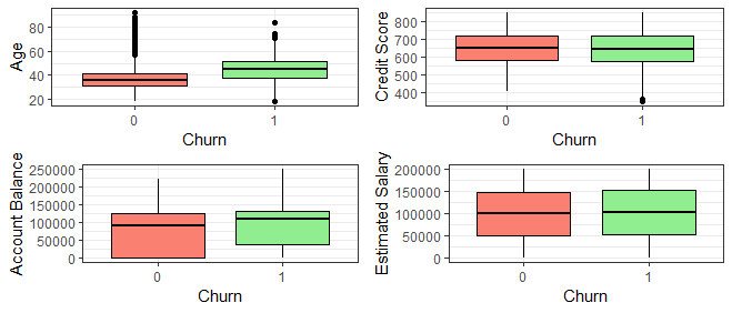
From our boxplot above, there is no significant correlation between churn and our other variables: age, credit score, account balance and estimated salary, indicating a complex interplay of factors that lead to a customer churning or not.
Unveiling Insights Through Visuals
In our exploratory data analysis, several key insights emerge from the visualizations. The customer age distribution depicts a youthful base, with the majority below 45 years and a noticeable decline in customers over 50 years. The symmetric distribution of credit scores highlights a concentration around the median score of 650, with a gradual tapering towards the extremes. Subsequent visualization of account balances initially reveals an unusually high number of zero balances, leading us to filter them out for clarity. This replotting indicates a right-skewed distribution with a peak around the median balance of 119,840, reflecting the diversity in customers' financial positions.
A symmetrical histogram of estimated salaries showcases a central tendency around the median value around 101,000, capturing the balanced representation of income levels within the dataset. When examining customers' distribution across countries, we find France to be the dominant country, followed by Germany and Spain. The bar chart depicting bank products ownership emphasizes a preference for fewer products among customers. The prevalence of credit card ownership suggests its significance in maintaining banking relationships, prompting deeper churn analysis to understand its link with customer engagement and retention potential. Moreover, an intriguing observation arises from the comparison of churn across countries, with Germany's unexpectedly high churn rate warranting further investigation.
Furthermore, gender-based churn analysis indicates a higher churn rate among females despite their lesser representation in the customer base. Lastly, our boxplot reveals that there is no significant correlation between churn and variables such as age, credit score, account balance, and estimated salary. This suggests a complex interplay of factors influencing churn, underscoring the need for a comprehensive approach. As we look ahead, machine learning techniques can enable us to delve deeper into these complexities, helping us identify hidden patterns and predictive factors that contribute to customer churn, thus empowering the bank to devise effective strategies for customer retention and engagement.
Building a Baseline Model: Logistic Regression
Why Logistic Regression? Logistic regression is a crucial analytical tool that holds significant relevance in our churn prediction project. As we aim to predict customer churn, which involves identifying whether a customer will continue using our services or terminate their relationship with the bank, logistic regression offers a powerful way to model this binary outcome.
In the context of our dataset, where we have various customer attributes and behaviors as features, logistic regression can help us understand the relationship between these features and the likelihood of churn. By fitting a logistic regression model, we can estimate the probability of a customer churning based on their individual characteristics. This estimation enables us to rank customers by their propensity to churn, allowing the bank to prioritize resources for retaining those who are at higher risk of leaving.
Moreover, logistic regression provides insights into the strength and direction of the relationships between individual features and churn. We can identify which factors contribute the most to churn risk and uncover potential patterns or behaviors that are associated with higher or lower churn rates. This information is invaluable for the bank to make informed decisions about targeting specific interventions or strategies towards those customers who are more likely to churn.
Additionally, logistic regression's interpretability is a key advantage. The coefficients obtained from the logistic regression model provide a clear understanding of how each feature influences the odds of churn. This transparency aids in explaining the results to stakeholders and allows the bank to make data-driven decisions based on the insights gained.
Logistic regression is relevant to our churn project as it serves as a foundational tool for building predictive models that can assess customer churn risk, uncover important variables affecting churn, and guide strategic efforts towards customer retention.
        # Set a seed for reproducibility
        set.seed(321)

        # Split the data into 70% training and 30% testing
        split <- sample.split(df$churn, SplitRatio = 0.7)
        train <- subset(df, split == T)
        test <- subset(df, split == F)

        # Define predictor variables and the target variable
        predictors <- c(
                        "credit_score", "age", "tenure", "balance",
                        "products_number", "credit_card",
                        "active_member", "estimated_salary"
                    )

        target <- "churn"

        # Perform logistic regression
        m1 <- glm(
                formula = paste(target, "~", paste(predictors,
                                                            collapse = "+")),
                            family = "binomial", data = train
                )

        # Print summary of the model
        summary(m1)

        # Make predictions on the test data
        test_predictions <- predict(m1, newdata = test, type = "response")

        # Convert probabilities to binary predictions (0 or 1)
        test_predictions_binary <- ifelse(test_predictions > 0.5, 1, 0)
In this code snippet, we are performing logistic regression to predict customer churn. First, we set a seed for reproducibility using set.seed(321), sidenote: it can be any number you want. We then split the data into a training set (70%) and a testing set (30%) using the sample.split() function. Next, we define the predictor variables, such as credit score, age, tenure, balance, products owned, credit card ownership, active membership, and estimated salary. The target variable is set to "churn."
We use the glm() function to perform logistic regression. The formula is constructed using the target variable and the list of predictors, separated by the "+" symbol. The model is specified with the "binomial" family, indicating logistic regression, and the data is set to the training set. The summary() function provides a summary of the logistic regression model, displaying information about the coefficients, their estimates, standard errors, z-values, and p-values. The summary output presents details about the model's performance, including coefficients, estimates, and their significance levels. Each coefficient represents the change in the log odds of the target variable due to a unit change in the corresponding predictor variable. Significance levels are indicated by the number of asterisks (*), with more asterisks indicating higher significance.
Call:
glm(formula = paste(target, "~", paste(predictors, collapse = "+")),
    family = "binomial", data = train)

Deviance Residuals:
    Min       1Q   Median       3Q      Max
-2.6209  -0.6034  -0.3866  -0.1988   3.1488

Coefficients:
                    Estimate     Std. Error z value             Pr(>|z|)
(Intercept)       -3.1838762062   0.3551259716  -8.965 < 0.0000000000000002 ***
credit_score      -0.0008547481   0.0003565675  -2.397              0.01652 *
age                0.0715720554   0.0032244970  22.196 < 0.0000000000000002 ***
tenure1           -0.0393694130   0.1893473216  -0.208              0.83529
tenure2           -0.0294995883   0.1932104761  -0.153              0.87865
tenure3           -0.2112033254   0.1939147687  -1.089              0.27609
tenure4           -0.0402537203   0.1932911268  -0.208              0.83503
tenure5           -0.1121986003   0.1937782300  -0.579              0.56259
tenure6           -0.0880123772   0.1931244977  -0.456              0.64859
tenure7           -0.2212818046   0.1943304722  -1.139              0.25483
tenure8           -0.2412513321   0.1938921103  -1.244              0.21341
tenure9           -0.1444434904   0.1925091626  -0.750              0.45306
tenure10           0.0344467507   0.2220057783   0.155              0.87669
balance            0.0000034853   0.0000012680   2.749              0.00598 **
products_number2  -1.4663302408   0.0806341217 -18.185 < 0.0000000000000002 ***
products_number3   2.5389531522   0.2036242251  12.469 < 0.0000000000000002 ***
products_number4  16.5050844342 223.1247742135   0.074              0.94103
credit_card1      -0.0491406059   0.0748651358  -0.656              0.51157
active_member1    -1.1218524566   0.0733756810 -15.289 < 0.0000000000000002 ***
estimated_salary   0.0000007379   0.0000006044   1.221              0.22213
---
Signif. codes:  0 ‘***’ 0.001 ‘**’ 0.01 ‘*’ 0.05 ‘.’ 0.1 ‘ ’ 1

(Dispersion parameter for binomial family taken to be 1)

    Null deviance: 7077.1  on 6999  degrees of freedom
Residual deviance: 5385.8  on 6980  degrees of freedom
AIC: 5425.8

Number of Fisher Scoring iterations: 14
Our logistic regression model shows the variables that significantly impact the prediction of customer churn. Assessing the p-values associated with each variable aids in identifying the most impactful predictors. Notably, variables like credit_score and age display remarkably low p-values, highlighting their strong link to churn prediction. Furthermore, balance and the count of products_number show statistical significance, indicating that customers' financial status and engagement with multiple products are pivotal in determining the likelihood of churn. The active_member status emerges as highly significant, emphasizing the role of customer engagement in curbing churn risk.
On the contrary, certain variables like specific tenure periods, credit_card ownership, and products_number4 yield higher p-values, suggesting their less pronounced influence on churn. These findings provide a succinct yet informative overview of the primary predictors guiding customer churn.
In summary, a higher credit score is linked to a decreased probability of churn, suggesting that customers with stronger financial profiles are more inclined to remain with the bank. In contrast, younger customers appear more likely to churn, indicating a potential trend in this demographic. Interestingly, the number of products a customer holds seems to correlate with an increased likelihood of churn, while being an active member is significantly correlated with a reduced probability of churning.
        # Evaluate the model's performance
        conf_matrix <- confusionMatrix(table(test_predictions_binary, test$churn))
        print(conf_matrix)

        # Calculate accuracy, precision, recall, and F1-score
        accuracy <- conf_matrix$overall["Accuracy"] * 100
        precision <- conf_matrix$byClass["Pos Pred Value"] * 100
        recall <- conf_matrix$byClass["Sensitivity"] * 100
        f1_score <- conf_matrix$byClass["F1"] * 100

        # Print evaluation metrics
        print(paste("Accuracy:", accuracy, "%"))
        print(paste("Precision:", precision, "%"))
        print(paste("Recall:", recall,"%"))
        print(paste("F1-Score:", f1_score, "%"))
The model is trained on a training dataset and used on a testing dataset to make predictions. The performance metrics we will use to evaluate our baseline and comparison models are: accuracy, precision, recall, and F1-score.
The choice of performance metrics plays a critical role in evaluating the effectiveness of machine learning models, both in the context of logistic regression and random forests. These metrics allow us to quantitatively assess how well our models are performing and provide a comprehensive understanding of their predictive capabilities.
Accuracy is a fundamental metric that measures the proportion of correctly classified instances out of the total instances in the dataset. It provides a general overview of a model's overall correctness but can be misleading in cases where class distribution is imbalanced.
Precision focuses on the true positive rate among the instances that the model classifies as positive. It helps us understand the accuracy of positive predictions and is particularly useful when the cost of false positives is high, such as in medical diagnoses or fraud detection, and in our case, predicting whether the bank will lose business or retain it.
Recall, also known as sensitivity or true positive rate, measures the proportion of actual positive instances that the model correctly identifies as positive. It is crucial when the cost of false negatives is high, as in cases where missing a positive case has significant consequences.
F1-score is the harmonic mean of precision and recall, providing a balanced measure of a model's performance. It is especially valuable when we want to strike a balance between precision and recall.
These performance metrics collectively allow us to comprehensively assess the strengths and weaknesses of both logistic regression and random forests models. By considering multiple metrics, we can make more informed decisions about model selection, fine-tuning, and optimization to achieve the desired trade-offs between accuracy, precision, recall, and F1-score based on the specific goals of our churn prediction project.
Upon evaluating the performance of our model, a confusion matrix is utilized to provide a comprehensive overview of its predictive capabilities. The matrix presents the counts of true positive, true negative, false positive, and false negative predictions, facilitating a clear assessment of the model's effectiveness.
        Confusion Matrix and Statistics


        test_predictions_binary    0    1
                            0 2310  425
                            1   79  186

                    Accuracy : 0.832
                        95% CI : (0.8181, 0.8452)
            No Information Rate : 0.7963
            P-Value [Acc > NIR] : 0.0000003956

                        Kappa : 0.3438

        Mcnemar's Test P-Value : < 0.00000000000000022

                    Sensitivity : 0.9669
                    Specificity : 0.3044
                Pos Pred Value : 0.8446
                Neg Pred Value : 0.7019
                    Prevalence : 0.7963
                Detection Rate : 0.7700
        Detection Prevalence : 0.9117
            Balanced Accuracy : 0.6357

            'Positive' Class : 0

        >
        > # Calculate accuracy, precision, recall, and F1-score
        > accuracy <- conf_matrix$overall["Accuracy"] * 100
        > precision <- conf_matrix$byClass["Pos Pred Value"] * 100
        > recall <- conf_matrix$byClass["Sensitivity"] * 100
        > f1_score <- conf_matrix$byClass["F1"] * 100
        >
        > # Print evaluation metrics
        > print(paste("Accuracy:", accuracy, "%"))
        [1] "Accuracy: 83.2 %"
        > print(paste("Precision:", precision, "%"))
        [1] "Precision: 84.4606946983547 %"
        > print(paste("Recall:", recall,"%"))
        [1] "Recall: 96.693177061532 %"
        > print(paste("F1-Score:", f1_score, "%"))
        [1] "F1-Score: 90.1639344262295 %"
The confusion matrix for our churn logistic regression model provides a visual representation of the model's classification performance on the test dataset. The matrix is organized into four quadrants, each representing different outcomes based on the predicted and actual class labels.
In the upper left quadrant, we have the True Negatives (TN), which are instances correctly predicted as the negative class (no churn). In this case, there are 2310 instances where the model correctly predicted no churn, aligned with the actual negative class.
In the lower right quadrant, we find the True Positives (TP), representing instances correctly predicted as the positive class (churn). Here, the model accurately predicted 186 instances of churn, matching the actual positive class.
The upper right quadrant contains False Positives (FP), indicating instances that were predicted as churn but actually belonged to the no churn class. In this case, there are 425 instances that were falsely predicted as churn when they were not.
Finally, the lower left quadrant represents False Negatives (FN), which are instances that were predicted as no churn but were actually churn cases. The model incorrectly predicted 79 instances as no churn when they were actually churn.
Additionally, various statistics are computed to gauge the model's overall performance. The accuracy of 83.2% demonstrates the proportion of correct predictions among the total predictions made. Precision, denoting the accuracy of positive predictions, is calculated at 84.46%, signifying the model's capability to correctly identify positive cases. The recall rate, measuring the ability to capture all actual positive cases, stands at an impressive 96.69%. Moreover, the F1-Score, a balanced metric considering both precision and recall, is determined to be 90.16%. These evaluation metrics collectively provide insights into the model's strengths and weaknesses. The high recall suggests that the model is adept at identifying customers who are likely to churn, while the precision indicates that the majority of predicted churns are indeed accurate. The F1-Score showcases a balanced combination of precision and recall, illustrating the model's overall reliability. These metrics play a pivotal role in assessing the model's suitability for real-world applications, guiding businesses in making informed decisions about their customer retention strategies and ensuring efficient resource allocation.
We will then go on to draw a comparison model using the Random Forest algorithm and evaluate its performance against that of our aforementioned logistic regression model.
Building a Comparison Model: Random Forest.
To have a comparison model for our churn prediction, we also implement a Random Forest model.
Random Forest is a powerful machine learning algorithm that holds great relevance for our churn prediction project. It's like an ensemble of decision trees, where each tree learns patterns from different subsets of data. This approach helps mitigate overfitting and improves prediction accuracy. In our context, Random Forest can effectively learn and capture complex relationships between various factors influencing customer churn.
Random Forest is particularly suitable for our comparison model due to its versatility and robustness. It handles both categorical and numerical features well, making it suitable for our dataset with diverse variables like age, credit score, and product ownership. Its ability to identify important features helps us understand the most influential factors affecting churn, as highlighted in feature importance scores. Additionally, Random Forest is less prone to overfitting compared to individual decision trees, ensuring that our model generalizes well to new data.
        # Train the Random Forest model
        rf_model <- randomForest(churn ~ ., data = train[, c(
                predictors, "churn")])

        # Make predictions on the test set
        rf_predictions <- predict(rf_model, test[, c(predictors, "churn")])
Here, we are training a Random Forest model. Random Forests learn patterns from data to make predictions. In this case, we're trying to predict the "churn" variable, which indicates whether a customer will leave the bank (churn = 1) or not (churn = 0). We're using the randomForest function, and the formula churn ~ . indicates that we want to predict "churn" using all the other variables in the dataset. The data used for training is taken from the "train" dataset, which includes the columns specified in "predictors" (other variables that might influence churn) and the "churn" column.
After training the model, we want to see how well it can predict on new, unseen data. This is where the "test" dataset comes in. We use the trained rf_model to predict the churn outcomes for the test data. The predict function takes the trained model and the data we want to predict on, our test dataset. The predictions are stored in the variable rf_predictions.
        # Model diagnostics
        summary(rf_model)
                        Length Class  Mode
        call                3  -none- call
        type                1  -none- character
        predicted        7000  factor numeric
        err.rate         1500  -none- numeric
        confusion           6  -none- numeric
        votes           14000  matrix numeric
        oob.times        7000  -none- numeric
        classes             2  -none- character
        importance          8  -none- numeric
        importanceSD        0  -none- NULL
        localImportance     0  -none- NULL
        proximity           0  -none- NULL
        ntree               1  -none- numeric
        mtry                1  -none- numeric
        forest             14  -none- list
        y                7000  factor numeric
        test                0  -none- NULL
        inbag               0  -none- NULL
        terms               3  terms  call
# Evaluate the model's performance
conf_matrix_rf <- confusionMatrix(table(rf_predictions, test$churn))
accuracy_rf <- conf_matrix_rf$overall["Accuracy"] * 100
precision_rf <- conf_matrix_rf$byClass["Pos Pred Value"] * 100
recall_rf <- conf_matrix_rf$byClass["Sensitivity"] * 100
f1_score_rf <- conf_matrix_rf$byClass["F1"] * 100
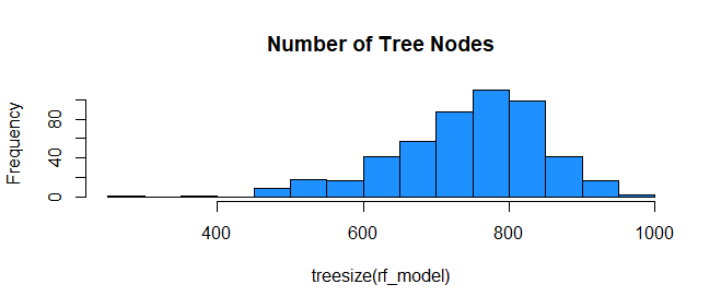
# model tree node distribution
hist(treesize(rf_model), col="dodgerblue",
main = "Number of Tree Nodes")
# Get variable importance from the Random Forest model
variable_importance_rf <- importance(rf_model)
# Print the variable importance
print("Random Forest Variable Importance:")
print(variable_importance_rf)
varImpPlot(rf_model)
# Print evaluation metrics
print(paste("Random Forest Model Metrics:"))
print(paste("Accuracy:", accuracy_rf, "%"))
print(paste("Precision:", precision_rf, "%"))
print(paste("Recall:", recall_rf, "%"))
print(paste("F1-Score:", f1_score_rf, "%"))
        > # Print the variable importance
        > print("Random Forest Variable Importance:")
        [1] "Random Forest Variable Importance:"
        > print(variable_importance_rf)
                        MeanDecreaseGini
        credit_score            266.85015
        age                     512.61482
        tenure                  193.99792
        balance                 267.20109
        products_number         284.01493
        credit_card              32.88882
        active_member            87.88328
        estimated_salary        266.65760
        > varImpPlot(rf_model)
        >
        > # Print evaluation metrics
        > print(paste("Random Forest Model Metrics:"))
        [1] "Random Forest Model Metrics:"
        > print(paste("Accuracy:", accuracy_rf, "%"))
        [1] "Accuracy: 84.6666666666667 %"
        > print(paste("Precision:", precision_rf, "%"))
        [1] "Precision: 85.9485650391353 %"
        > print(paste("Recall:", recall_rf, "%"))
        [1] "Recall: 96.5257429886982 %"
        > print(paste("F1-Score:", f1_score_rf, "%"))
        [1] "F1-Score: 90.9305993690852 %"
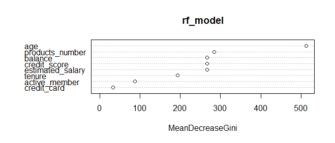
The insights drawn from the MeanDecreaseGini values have direct implications for predicting customer churn in the context of a bank's operations. Notably, age emerges as a leading influencer, boasting a significant score of 512.61. This observation indicates that age-related trends and behaviors play a pivotal role in shaping the model's predictions regarding customer churn.
Similarly, variables like products number, balance, credit score, and estimated salary, each exhibiting values in the range of 266 to 284, underscore their considerable impact on the model's decision-making process. These attributes likely encapsulate critical aspects of customers' financial standings and interactions with the bank.
Conversely, variables like active membership, tenure, and credit card usage, despite their relatively lower MeanDecreaseGini values, still contribute meaningfully to the model's predictive capability. Their inclusion in the model's architecture, albeit with slightly diminished influence, highlights their role in predicting customer churn. By delving into the nuances of variable importance, a strategic approach comes to the forefront, guiding feature selection, model refinement, and a deeper comprehension of the driving forces behind customer behaviors and outcomes. This understanding holds significant value in shaping effective strategies to mitigate churn within the specific context of the bank's customer dataset.
The reported metrics include accuracy, precision, recall, and the F1-score. Accuracy, at about 84.67%, indicates the proportion of correctly predicted instances. Precision, approximately 85.95%, outlines the proportion of true positive predictions among positive predictions. Recall, standing at around 96.53%, signifies the proportion of actual positives that were accurately predicted. Lastly, the F1-score, around 90.93%, harmonizes precision and recall to offer a balanced view of the model's performance. These metrics collectively offer a comprehensive assessment of the model's predictive prowess and its ability to handle different aspects of the classification task.
The comparison between the logistic regression model (`m1`) and the Random Forest model (`rf_model`) for predicting customer churn produced the corresponding evaluation results.
The logistic regression model yielded the following evaluation metrics on the test data:
- Accuracy: 83.2%
- Precision: 84.46%
- Recall: 96.69%
- F1-Score: 90.16%
The Random Forest model produced the following evaluation metrics on the same test data:
- Accuracy: 84.7%
- Precision: 85.95%
- Recall: 96.57%
- F1-Score: 90.95%
Comparing the metrics, the Random Forest model generally outperforms the logistic regression model across all evaluation aspects. It achieves a slightly higher accuracy, precision, recall, and F1-Score. This suggests that the Random Forest model is better suited for this specific customer churn prediction task, as it provides improved predictive capabilities compared to the logistic regression model. The Random Forest model's higher performance could be attributed to its ability to capture complex relationships between predictor variables, handle interactions, and handle non-linearities effectively, which can be particularly advantageous when dealing with intricate patterns in customer churn behavior.
Conclusion
Predicting customer churn is a crucial task for businesses aiming to retain their valuable customers. By harnessing the power of data analysis and machine learning techniques, we can uncover patterns and insights from customer data that aid in making informed decisions.
In this article, we walked through the process of preparing and exploring the data, building predictive models, and interpreting the results.
Our exploration into churn prediction models offers valuable insights for businesses, especially banks, striving to address customer attrition. Through two distinct models, logistic regression and Random Forest, we gain a deeper understanding of the factors that influence customers' decisions to churn. Logistic regression highlights the significance of variables such as credit score, age, tenure, balance, products owned, active membership, and estimated salary in predicting churn likelihood. On the other hand, the Random Forest model emphasizes the importance of age, products owned, balance, and credit score as key predictors of churn. These insights equip businesses with the knowledge needed to create targeted strategies for customer retention.
The role of machine learning in comprehending churn dynamics extends across industries. By analyzing large datasets, these models uncover intricate patterns and forecast churn with remarkable accuracy, enabling businesses to adopt proactive retention measures. This shift from reactive to proactive churn management offers benefits beyond banking, extending to sectors like retail, telecommunications, and subscription services. By tailoring their approaches, businesses can elevate customer experiences, foster brand loyalty, and bolster their financial performance.
In conclusion, the amalgamation of predictive models and the capabilities of machine learning brings about a transformative change in the way we approach churn. Armed with insights into critical variables, businesses can optimize their strategies to enhance engagement, minimize attrition, and cultivate lasting customer relationships. As organizations embrace the potential of machine learning, gaining an intimate understanding of churn emerges as a cornerstone for achieving sustainable growth and thriving in today's competitive landscape.